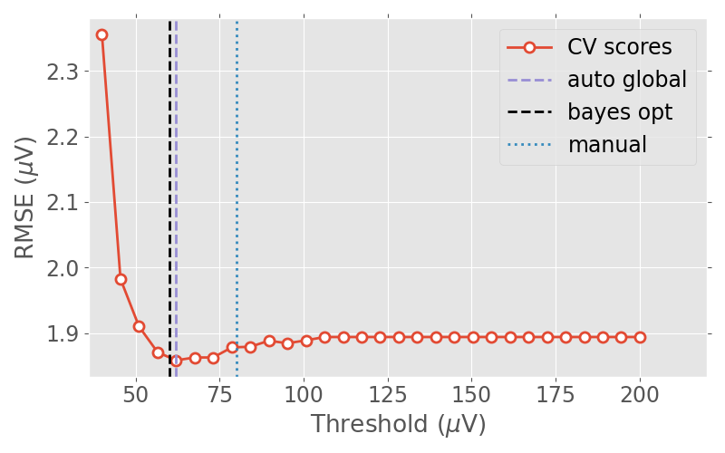
Plotting the cross-validation curve

This example demonstrates how to use autoreject to plot the cross-validation curve that is used to estimate the global rejection thresholds.

# Author: Mainak Jas <mainak.jas@telecom-paristech.fr>
# License: BSD-3-Clause

Let us import the data using MNE-Python and epoch it.

import mne
from mne import io
from mne.datasets import sample

event_id = {'Visual/Left': 3}
tmin, tmax = -0.2, 0.5

data_path = sample.data_path()
meg_path = data_path / 'MEG' / 'sample'
raw_fname = meg_path / 'sample_audvis_filt-0-40_raw.fif'
event_fname = meg_path / 'sample_audvis_filt-0-40_raw-eve.fif'

raw = io.read_raw_fif(raw_fname, preload=True)
events = mne.read_events(event_fname)

include = []
picks = mne.pick_types(raw.info, meg=False, eeg=True, stim=False,
                       eog=False, include=include, exclude='bads')
epochs = mne.Epochs(raw, events, event_id, tmin, tmax,
                    picks=picks, baseline=(None, 0),
                    reject=None, verbose=False, detrend=1)

Opening raw data file C:\Users\stefan\mne_data\MNE-sample-data\MEG\sample\sample_audvis_filt-0-40_raw.fif...
    Read a total of 4 projection items:
        PCA-v1 (1 x 102)  idle
        PCA-v2 (1 x 102)  idle
        PCA-v3 (1 x 102)  idle
        Average EEG reference (1 x 60)  idle
    Range : 6450 ... 48149 =     42.956 ...   320.665 secs
Ready.
Reading 0 ... 41699  =      0.000 ...   277.709 secs...

Let us define a range of candidate thresholds which we would like to try. In this particular case, we try from \(40{\mu}V\) to \(200{\mu}V\)

import numpy as np  # noqa
param_range = np.linspace(40e-6, 200e-6, 30)

Next, we can use autoreject.validation_curve() to compute the Root Mean Squared (RMSE) values at the candidate thresholds. Under the hood, this is using autoreject._GlobalAutoReject to find global (i.e., for all channels) peak-to-peak thresholds.

from autoreject import validation_curve  # noqa
from autoreject import get_rejection_threshold  # noqa

_, test_scores, param_range = validation_curve(
    epochs, param_range=param_range, cv=5, return_param_range=True, n_jobs=1)

test_scores = -test_scores.mean(axis=1)
best_thresh = param_range[np.argmin(test_scores)]

Using data from preloaded Raw for 73 events and 106 original time points ...
0 bad epochs dropped

We can also get the best threshold more efficiently using Bayesian optimization

reject2 = get_rejection_threshold(epochs, random_state=0, cv=5)

Using data from preloaded Raw for 73 events and 106 original time points ...
Estimating rejection dictionary for eeg

Now let us plot the RMSE values against the candidate thresholds.

import matplotlib.pyplot as plt  # noqa
from autoreject import set_matplotlib_defaults  # noqa
set_matplotlib_defaults(plt)

human_thresh = 80e-6  # this is a threshold determined visually by a human
unit = r'$\mu$V'
scaling = 1e6

plt.figure(figsize=(8, 5))
plt.tick_params(axis='x', which='both', bottom='off', top='off')
plt.tick_params(axis='y', which='both', left='off', right='off')

colors = ['#E24A33', '#348ABD', '#988ED5', 'k']

plt.plot(scaling * param_range, scaling * test_scores,
         'o-', markerfacecolor='w',
         color=colors[0], markeredgewidth=2, linewidth=2,
         markeredgecolor=colors[0], markersize=8, label='CV scores')
plt.ylabel('RMSE (%s)' % unit)
plt.xlabel('Threshold (%s)' % unit)
plt.xlim((scaling * param_range[0] * 0.9, scaling * param_range[-1] * 1.1))
plt.axvline(scaling * best_thresh, label='auto global', color=colors[2],
            linewidth=2, linestyle='--')
plt.axvline(scaling * reject2['eeg'], label='bayes opt', color=colors[3],
            linewidth=2, linestyle='--')
plt.axvline(scaling * human_thresh, label='manual', color=colors[1],
            linewidth=2, linestyle=':')
plt.legend(loc='upper right')
plt.tight_layout()
plt.show()